The Girl with the Brick Earring
LEGO!
Who didn’t play with LEGO in his/her childhood? The Danish toy company just overtook Mattel as the number one toy maker in the world. I recently came across some classical paintings remodeled with LEGO bricks on the internet [citation needed]. And with bricks I mean small 1x1 plates giving a pixelated view onto the old masterpieces. Which got me thinking about two things: Is it possible to remodel any old classic into a LEGO version of itself? And: Can you do it only with colors already available for purchase? The last thing is important if you want to actually build the image after remodeling it. The examples I have found used a lot of colors not in the standard LEGO color palette.
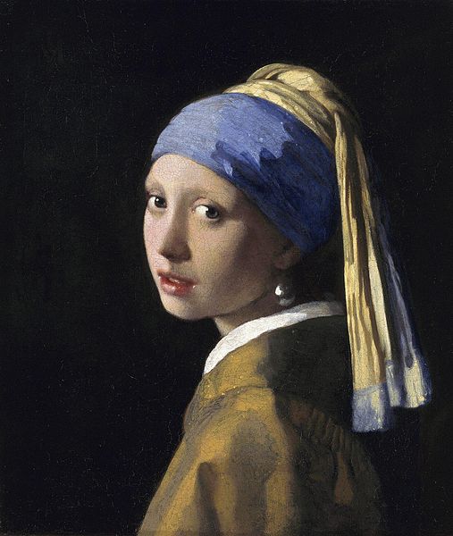
But first, let’s have a look at the original I have chosen. It is The Girl with the Pearl Earring by Johannes Vermeer.
The internet is made for … arbitrary table layouts
First things first. One of the first problems to tackle is the range of colors available. This was the first time I stumbled across Bricklink, a shop site offering single bricks for purchase. Trust me: They are great! And this is not the last time you will hear about them in this post (Trust me!). Bricklink offers a full color table. The good news: The table offers a timeline for each color and therefore the possibility to filter colors which are not available any more. The bad news: HTML crawling is necessary. Yay! So let’s set up a color table in a pandas DataFrame.
We import all the basic stuff for HTML crawling. Requests for downloading, BeautifulSoup for CSS selection and pandas for storing the table.
import requests
from bs4 import BeautifulSoup
import pandas as pd
Download the color table website…
headers = {
    'User-Agent': "Mozilla/5.0"
}

r = requests.get("https://www.bricklink.com/catalogColors.asp", headers=headers)
…and parse the information.
# helper function; translates hexcodes to integers
def hextoint(hexcode):
    return (int(hexcode[:2], 16), int(hexcode[2:4], 16), int(hexcode[4:], 16))

tree = BeautifulSoup(r.text, "lxml")

# select the fourth table in the HTML for solid colors
html_table = tree.select("table")[3].select("table")[0]
# let pandas read the table
color_table = pd.read_html(str(html_table), header=0)[0]
color_table = color_table.drop(["Unnamed: 1", "Unnamed: 2"] , axis=1)
# select the RGB values from the HTML background color and build three new columns with them
rgb_table = pd.DataFrame([hextoint(td.attrs["bgcolor"]) for td in html_table.select("td[bgcolor]")],
                         columns=["r", "g", "b"])
color_table = color_table.merge(rgb_table, left_index=True, right_index=True)
# select colors which are available in 2017 and which are not rare to find
current_colors = color_table[color_table["Color Timeline"].str.contains("2017")]
current_colors = current_colors[~(current_colors["Name"].str.contains("Flesh")
                                    | current_colors["Name"].str.contains("Dark Pink")
                                    | (current_colors["Name"] == "Lavender")
                                    | current_colors["Name"].str.contains("Sand Blue"))]
You might have noticed that I removed some colors by hand. Those are the colors which are so rare, they score up to 4.00€ per piece on Bricklink. If you still want them in your picture just remove the last instruction. So, current_colors should look like this. It contains circa 30 colors.
| ID | Name | Parts | In Sets | Wanted | For Sale | Color Timeline | r | g | b | |
|---|---|---|---|---|---|---|---|---|---|---|
| 0 | 1 | White | 9153.0 | 7306.0 | 10322 | 9104 | 1950 - 2017 | 255 | 255 | 255 |
| 3 | 86 | Light Bluish Gray | 2668.0 | 3993.0 | 4215 | 3002 | 2003 - 2017 | 175 | 181 | 199 |
| 6 | 85 | Dark Bluish Gray | 2404.0 | 3784.0 | 3673 | 2623 | 2003 - 2017 | 89 | 93 | 96 |
| ... | ... | ... | ... | ... | ... | ... | ... | ... | ... | ... |

50 Shades of LEGO
The following progress is called color quantisation. It replaces all colors with a limited choice of other colors. In our case the image pixels will be transmuted (+1 on the fancy word scale) to the LEGO color scale. This is done by finding the nearest neighbours in the RGB space. Each pixel is represented as a vector of its R, G and B component. The distance between two pixels is the euclidean distance between their respective vectors.
from sklearn.neighbors import NearestNeighbors
import numpy as np

# fit the NN to the RGB values of the colors; only one neighbour is needed
nn = NearestNeighbors(n_neighbors=1, algorithm='brute')
nn.fit(current_colors[["r", "g", "b"]])

# helper function; finds the nearest color for a given pixel
def pic2brick(pixel, nn, colors):
    new_pixel = nn.kneighbors(pixel.reshape(1, -1), return_distance=False)[0][0]
    return tuple(colors.iloc[new_pixel, -3:])
Now we replace all the pixels in the original (girl.jpg) with colors from current_colors.
from PIL import Image, ImageFilter

image = Image.open("girl.jpg")

# get a 10th of the image dimensions and the aspect ratio
w10 = int(image.size[0]/10)
h10 = int(image.size[1]/10)
ratio = image.size[0]/image.size[1]
# smooths the image and scales it to 20%
pixelated = image.filter(ImageFilter.MedianFilter(7)).resize((2*w10,2*h10))
# Quantise!
pixelated = np.array(pixelated)
pixelated = np.apply_along_axis(pic2brick, 2, pixelated, nn, current_colors)
pixelated = Image.fromarray(np.uint8(pixelated), mode="RGB")
# reduce the size of the image according to aspect ratio (32,x)
if ratio < 1:
    h = 32
    w = int(32*ratio)
else:
    w = 32
    h = int(32/ratio)
final = pixelated.resize((w,h))
final_arr = np.array(final) # image as array
After all this, the image (rescaled to the original’s size) looks like this. Isn’t she a looker?
![]()
Notes: If you use the fleshy colors, you will get a more even skin tone. You can see that the reduced color palette is far from perfect for classical images.
After generating an XML file for Bricklink’s upload-to-purchase tool (account required)…
from collections import defaultdict

order = defaultdict(int)
xml_string = "<INVENTORY>"
item_string = """<ITEM>
<ITEMTYPE>P</ITEMTYPE>
<ITEMID>3024</ITEMID>
<COLOR>{}</COLOR>
<MINQTY>{}</MINQTY>
</ITEM>"""

for pixel in final.getdata():
    row = nn.kneighbors(np.array(pixel).reshape(1, -1), return_distance=False)[0][0]
    order[current_colors.iloc[row, 0]] += 1

for col, num in order.items():
    xml_string += item_string.format(col, num)

xml_string += "</INVENTORY>"
print(xml_string)
…one can see that filling a image with only 1x1 plates (part ID: 3024) costs a rather large amount of money. For me, it was between 65€ and 103€ depending on the shop. This should make it clear to the reader, why I have chosen to shrink the image to 32 pixels. Any size larger would only cost more. But is there a way, not to Amarillo, but to enlarge the portions of the image with the same color? LEGO bricks and plates are rectangular most of the time. Can we fit rectangles larger than 1x1 into the image? Spoiler!
I’ll make my own algorithm. With blackjack and graphs!
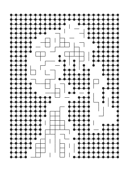
Fitting larger rectangles into the image should be easy. Just find all areas with the same color. Then, try to fill the areas with large rectangles. Let’s transfer the image to a graph. Every pixel is translated to a node with the x and y coordinates as positions in the graph and the color as a node property.
import networkx as nx

new_p = np.zeros((final.size))
G = nx.Graph()
pos = {} # positioning for plotting
colors = {} # colors for plotting
i = 0

for x in range(final.size[1]):
    for y in range(final.size[0]):
        G.add_node(str(x)+"|"+str(y), x=x, y=y)
        colors[str(x)+"|"+str(y)] = final_arr[x,y]/255
        pos[str(x)+"|"+str(y)] = [y,32-x]
        i += 1

        if x!=0 and np.array_equal(final_arr[x,y], final_arr[x-1,y]):
            G.add_edge(str(x)+"|"+str(y), str(x-1)+"|"+str(y))

        if y!=0 and np.array_equal(final_arr[x,y], final_arr[x,y-1]):
            G.add_edge(str(x)+"|"+str(y), str(x)+"|"+str(y-1))
The final graph looks a little bit like the original image, if you really squint your eyes.

You might have noticed the connections between the areas with the same color. Every pixel (or node) is connected to its neighbour if their color is the same. So, every enclosed color builds a connected component in the graph. The biggest one, as shown below, is of course the black background.
Now the tricky part begins. We fill all connected components of the graph with rectangles as large as possible. Therefore, the algorithm starts with the minimum node (left upper corner of an area) and expands southwards until the edge of the area is found or the maximum size is reached. Afterwards, it tries to expand the area eastwards with the same conditions. If an edge is found or the maximum size is reached the last complete rectangle is returned. The following video details the steps for the first black rectangle.
The function find_rectangles returns the complete set of rectangles over all connected components for the image.
def find_rectangles(G, max_size=12):
    assert max_size % 2 == 0 or max_size < 4, "Even numbers for max_size only!"
    bad_dims = set([5, 7, 9, 11, 13])
    all_rectangles = []

    # all connected subgraphs
    for gr in nx.algorithms.connected_component_subgraphs(G):
        while list(gr.nodes()): # as long as there are nodes
            node = min(gr.nodes(), key=lambda x: [int(y) for y in x.split("|")]) # get min x,y
            rectangle = []
            count = 0

            # vertical edge (expand southwards) until bottom line of subgraph
            # or max size
            while node in gr and count <= max_size - 1:
                rectangle.append(node)
                x,y = node.split("|")
                node = "{}|{}".format(int(x)+1, y)
                # widths > 4 are: 6, 8, 10, 12, 14
                if count > 2:
                    if node in gr and count + 1 <= max_size - 1:
                        rectangle.append(node)
                        node = "{}|{}".format(int(x)+2, y)
                        count += 1
                count += 1

            # 5 and 3 are stupid numbers for LEGO plates,
            # 3 can only occur in one dimension,
            # 5 can never occur anywhere
            if count in bad_dims:
                rectangle.pop(-1)
            if count == 3:
                bloody_3 = True
            else:
                bloody_3 = False

            final_rectangle = rectangle

            border_found = False
            count = 0

            # horizontal edge (expand eastwards)
            while (not border_found):
                right_border = []
                for rect_node in rectangle:
                    x,y = rect_node.split("|")

                    node = "{}|{}".format(x, int(y)+1)
                    # widths > 4 are: 6, 8, 10, 12
                    if count > 2:
                        if node in gr and count + 1 <= max_size - 1:
                            right_border.append(node)
                            node = "{}|{}".format(x, int(y)+2)
                            count += 1
                    # found right border of color (not in subgraph)
                    # or reached max size
                    # or the first dimension is 3 and so the second dimension must be <= 3
                    # or the second dimension will be 3 (not possible)
                    if count == 1:
                        node_la = "{}|{}".format(x, int(y)+2)
                    if (node not in gr) or (count >= max_size - 1) or (bloody_3 and count > 1)\
                                        or (count == 1 and node_la not in gr):
                        gr.remove_nodes_from(final_rectangle)
                        all_rectangles.append(final_rectangle)
                        border_found = True
                        break
                    else:
                        right_border.append(node)

                if not border_found:
                    final_rectangle += right_border
                    rectangle = right_border
                    count += 1

    return all_rectangles

meh = find_rectangles(G, max_size=12)
max_size is used to control the maximum dimension of LEGO plates used. You can change it according to your likings. The full traversal looks like this:
Calling Billund (DK)
After collecting another HTML page with the mappings from brick sizes to part IDs,…
r = requests.get("https://www.bricklink.com/catalogList.asp?catType=P&catString=26", headers=headers)

tree = BeautifulSoup(r.text, "lxml")

html_table = tree.select("#ItemEditForm")[0].select("table")[1]
part_table = pd.read_html(str(html_table), header=0)[0]
part_table.drop("Image", axis=1, inplace=True)
part_table.columns = ["ID", "Description"]
part_table["Description"] = part_table["Description"].str.split("Cat").str[0].str[6:]
part_table = part_table[part_table["Description"].str.len() < 10]
…I’m able to collect a material list…
measures = []
plate_colors = []

for rect in meh:

    row = nn.kneighbors(np.array(colors[rect[0]]*255).reshape(1, -1), return_distance=False)[0][0]
    color = current_colors.iloc[row, 0]

    key_x = lambda x: int(x.split("|")[0])
    key_y = lambda y: int(y.split("|")[1])

    min_x = int(min(rect, key=key_x).split("|")[0])
    min_y = int(min(rect, key=key_y).split("|")[1])

    max_x = int(max(rect, key=key_x).split("|")[0])
    max_y = int(max(rect, key=key_y).split("|")[1])

    measures.append("{} x {}".format(min(max_x-min_x+1, max_y-min_y+1), max(max_x-min_x+1, max_y-min_y+1)))
    plate_colors.append(color)
..and build the final Bricklink XML.
order = defaultdict(int)
xml_string = "<INVENTORY>"
item_string = """<ITEM>
<ITEMTYPE>P</ITEMTYPE>
<ITEMID>{}</ITEMID>
<COLOR>{}</COLOR>
<MINQTY>{}</MINQTY>
</ITEM>"""

for plate, color in zip(measures, plate_colors):
    p_id = part_table[part_table["Description"] == plate]["ID"].values[0]
    order[str(p_id) + "|" + str(color)] += 1

for plate, num  in order.items():
    xml_string += item_string.format(*plate.split("|"), num)

xml_string += "</INVENTORY>"
print(xml_string)
The XML can now be uploaded to Bricklink and you can order all the parts there.
We built this city on LEGO
Let me summarise what I have accomplished.
- quantised and pixelated an image to make it look like it is made out of LEGO,
- intelligently reduced the number of bricks used via graph connectivity,
- having so much fun, I actually ordered the bricks (~30€) and built the image.
Yes, you read right: I built the image with actual LEGO bricks. So, the last thing for me to say is: Back to my hands, desperately trying to find that one piece, I saw earlier. Arrgh! Where is it?
Other sources and libraries include pillow, networkx and scikit-learn.